To sort a table with linked data

[jsx97]

There is a Numbers document with 3 sheets: first (2 columns), second (1 column), and third (1 column).

second:

sun
grass
sea

third:

yellow
green
blue

first:

Column A             | Column B
=second::Table 1::A1 | =third::Table 1::A1
=second::Table 1::A2 | =third::Table 1::A2
=second::Table 1::A3 | =third::Table 1::A3

which results to:

Column A | Column B
sun      | yellow
grass    | green
sea      | blue

Fine. But if I try to sort ascending the table on second sheet, grass become yellow, sea green, and sun blue:

Column A | Column B
grass    | yellow
sea      | green
sun      | blue

The same issue happens if I try to sort the table on the third sheet instead:

Column A | Column B
sun      | blue
grass    | green
sea      | yellow

What do I need to fix/workaround this issue?

I have read many forum threads at Apple Discussions and there were suggestions to use LOOKUP and INDIRECT functions, but I have not realized how to use them here and whether they are suitable for this particular case at all.

[cornchip]

Would it work to just Copy Snapshot of the values of table A and save that as a new sheet? INDIRECT and LOOKUP won’t help you if you don’t store the proper associations between these two lists somewhere.

[Denny]

If you want to link records across tables/sheets you need to have a second column in the tables on the second and third sheets. The 2nd column functions as an ID. Then in the sheet where you want to display the columns side by side you’ll enter the ID number and do a look-up. At least, that’s the way I would do it. Screenshots:

I actually did my example in a different order, the third sheet contains the table that displays the columns side by side. Doing it this way live links data between the three tables based on the ID. So if a new row is added to sheets 1 and 2, in my tables, the next would be 7, then adding a new row in sheet 3 with an ID of 7 will auto populate the columns.

It’s still not doing the sorting you want but I’m not sure that’s possible, at least, not in the way you are asking to do it.

[ehpehp]

Agree with Denny on using a common variable to link items in Table 2 and 3.

Something like this for Table 2 and 3, and the formula for Table 1’s column B as listed.

[Denny]

Oh, much better to illustrate it with all the tables together like that!

[jsx97]

Thank you so much. But unfortunately sorting still broken. After I sort the table on sheet2 or on the sheet3 (by column B in both cases), the table on sheet1 is messed up. I have uploaded a file here:

https://file.io/V3T47jYIRvjn

What is wrong with it?

[jsx97]

Just in case, here is another test file, with all 3 tables on the same sheet. Still doesn’t work.

https://file.io/6B8GJ76VvgF3

[Denny]

Looking at your file, you haven’t used the Number ID column on the third table. What you seem to want to do may not be possible. Using the unique number ID column is a way of tying records together across tables based on the number.

In my example I have two tables that use the ID field to assign values.

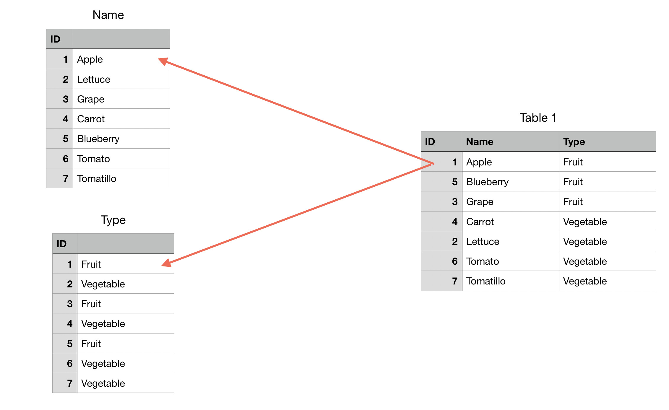
One table is called Name where we have the names of produce such as Apple, Carrot, Grape. The other table is called Type with two options fruit, vegetable.

Think of the number ID as being the primary key that all 3 tables use to talk to one another.

I populate the “Name” table with names of produce.

1, Apple
2, Lettuce
3, Grape
And so on

I then populate the “Type” table with the types of produce

1, Fruit
2, Vegetable
3, Fruit

Since 1 is assigned to Apple on the “Name” table, in the “Type” table I will give it a value of Fruit.

Since 2 is assigned to Lettuce on the “Name” table, in the “Type” table I will give it a value of Vegetable.

3 is assigned to Grape on the “Name” table, in the “Type” table I will give it a value of Fruit.

I work through each row of the “Type” table looking at the ID number then assign it the appropriate type based on the values in the “Name” table

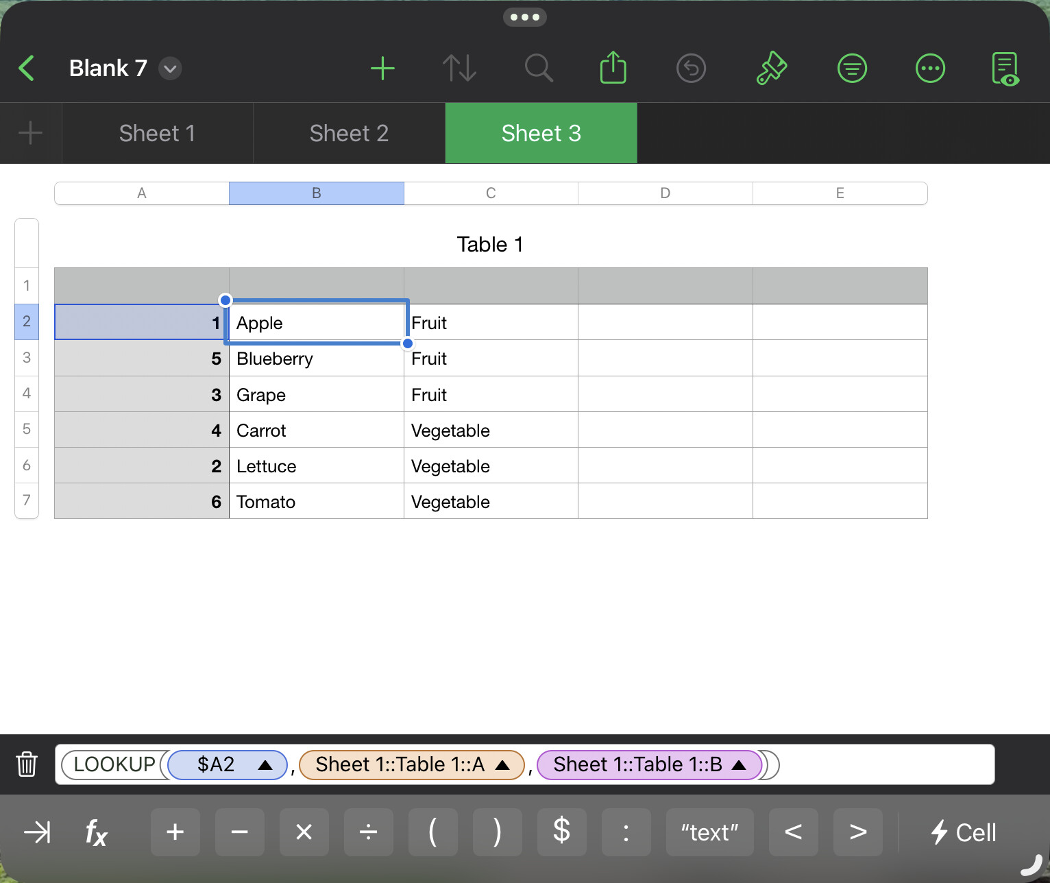
After those first two tables are populated with data I move onto the 3rd table. I start by adding 1 into my ID column. Then in the second column, “Name”, I do a Lookup. It’s going to look in the first column for the ID than it will search the “Name” table for the ID and then fill in the matching value in the Name column.

In the third column I do a Lookup also set up to look in the first column for the ID then it will search the “Type” table for the ID and will fill in the matching value in the Type column.

These two Lookups in the Name and Type columns should auto fill based on whatever number is in the first column. If I type in a 1 then I’ll get Apple, Fruit. If I type in a 2 it will fill to Lettuce, Vegetable. Once I have that row completed I can just hit return and a new row will be created with my Lookup formula intact. As soon as I type in the next ID it will auto fill based on the other two tables. Once I’ve added my 7 rows with the ID typed into each I’ll see all of my items have been auto filled. I can sort this table as needed. By ID, by Name or by Type.

Here’s the example file from iCloud.

[Denny]

Following up to just add, how you set-up really depends on what you’re after. Over the years I spent more time with FileMaker databases than spreadsheets. Of course, spreadsheets are a different way of doing things. But it can be helpful, especially if doing multi tables with linked data to think of it as a relational database. But it’s important to consider the desired functionality. In some cases multiple tables are needed, in some cases it might be better to have a single table with multiple columns.

In my example file, depending on use case, it would likely make more sense to do things very differently. To have a single table of Fruits that have multiple columns for different variables. I can imagine say a produce shop that would be tracking its current stock but in such a case it would probably make more sense to have a single table rather than the 3 in my example.

Again, it will depend on your use case and what you’re trying to do with the data.

[ehpehp]

In the test I created, I used this formula for Table 1’s cell A1 (and copied down to A3), not a lookup formula. This addresses Denny’s point. Sorting should work for all 3 tables without mismatching object and color.

[jsx97]

@Denny, thanks a lot! So it seems there is no way to reduce the Type table to 2 rows instead of 7, that is, to have only one “Fruit” and only one “Vegetable” rows there?